| Issue |
JNWPU
Volume 44, Number 1, February 2026
|
|
|---|---|---|
| Page(s) | 112 - 124 | |
| DOI | https://doi.org/10.1051/jnwpu/20264410112 | |
| Published online | 27 April 2026 | |
State estimation of DDS-DNNS with stochastic event-triggered mechanism under Bayes theory
Bayes理论下具有随机事件触发机制的DDS-DNNS状态估计
Coast Guard Academy, Naval Aviation University, Yantai, 264001, China
Received:
21
April
2025
Abstract
Addressing the state estimation problem of a single positioning node in a decentralized networked navigation system based on data distribution service(DDS-DNNS), considering node energy constraints and sensor gain degradation, a minimum mean square error(MMSE) state estimator for DDS-DNNS with a stochastic event-triggered(SET) mechanism is designed based on Bayesian theory. The SET mechanism determines the importance of measurement values by comparing the differences in posterior estimates corresponding to the transmitted measurement values. Based on this, the Wasserstein distance is selected as a metric to represent the difference in posterior estimates. The properties of the Wasserstein distance and Bayes' theorem are utilized to prove that the posterior estimate is Gaussian, thereby obtaining the Kalman-like filter recursive form of the estimator and the explicit expression of the SET mechanism. Subsequently, it is proven that the prediction error covariance of the estimator is bounded, and both the upper and lower bounds converge. Meanwhile, it is demonstrated that the average information transmission rate is bounded, and the expressions for the upper and lower bounds are derived. Finally, a numerical simulation is conducted to illustrate how to determine the adjustment matrix through the upper and lower bounds of the average information transmission rate. The impact of first-order moment information and second-order moment information on the SET mechanism is simulated, and the effectiveness of the estimator is verified through comparative experiments.
摘要
针对基于数据分发服务的分散式组网导航系统(decentralized networked navigation system based on DDS, DDS-DNNS)单定位节点状态估计问题, 考虑节点能量约束及传感器增益退化, 以Bayes理论为基础, 设计了具有随机事件触发机制(stochastic event-triggered, SET)的DDS-DNNS最小均方误差状态估计器。其中, SET机制通过比较是否传输测量值对应的后验估计的差异来决定测量值的重要程度。以此为基础, 选取Wasserstein距离作为度量来表示后验估计的差异, 并利用Wasserstein距离的性质及Bayes定理证明了后验估计是Gaussian的, 从而得到了估计器的类Kalman滤波递推形式以及SET机制的显式表达式。证明了估计器的预测误差协方差有界, 且上界和下界均收敛, 同时, 证明了平均信息传输率有界并推导得到了上界和下界的表达式。利用算例仿真演示了如何通过平均信息传输率的上界和下界确定调整矩阵, 模拟了SET机制中一阶矩信息和二阶矩信息对SET机制的影响, 同时采用比较实验验证了估计器的有效性。
Key words: Bayes theory / stochastic event-triggered / Kalman filter / posterior estimation / minimum mean square error state estimation
关键字 : Bayes理论 / 随机事件触发 / Kalman滤波 / 后验估计 / 最小均方误差状态估计
© 2026 Journal of Northwestern Polytechnical University. All rights reserved.
 This is an Open Access article distributed under the terms of the Creative Commons Attribution License (https://creativecommons.org/licenses/by/4.0), which permits unrestricted use, distribution, and reproduction in any medium, provided the original work is properly cited.
DDS-DNNS是一套自主研发的面向蜂群无人机局部定位需求的网络化导航系统[1]。在大规模组网情景下,DDS-DNNS所面临的组网压力主要体现在3个方面:①能量有限的电池使得无人机面临着严峻的能量约束[2-4];②有限的带宽资源随着数据包传输总量的增大而难以满足高质量通信需求[5-7];③DDS-DNNS传感器本身的增益退化导致估计器性能衰减[8]。
考虑到多个定位节点情景下,传感器与传感器之间测量值的交互会加剧上述三方面的压力,本文重点研究单个定位节点动态模型的估计器设计问题,后续将在此基础上进一步研究多节点融合估计器设计。
对于单个定位节点的状态估计器设计,需要重点考虑的是能量约束与传感器增益退化。文献[9]指出降低传感器到估计器的信息传输率能够有效缓解传感器的工作压力。因此,估计器需要通过设计判断准则筛选出对状态估计重要的信息。基于上述想法,文献[9]提到的事件触发(event-triggered, ET)机制将被应用至DDS-DNNS中,ET机制仅传输满足重要性度量的传感器测量值,有效地权衡了估计器性能和传感器工作压力。
对于ET机制中如何判断测量值的重要性程度,文献[10-14]设计了触发阈值为常数的ET机制,即确定性ET(deterministic event-triggered, DET)机制。DET机制下,传感器传输测量值至估计器当且仅当触发条件超过特定阈值。DET机制有效降低了传感器至估计器的信息传输率,但是,文献[10-14]设计的DET机制显然截断了新息序列的Gaussian概率密度函数(probability density function, PDF),导致难以获取准确的最小均方误差(minimum mean square error, MMSE)估计器。为此,文献[15]设计了基于新息的DET机制,该机制通过广义封闭偏正态分布推导得到,能够证明对应MMSE估计器的准确性。但是,文献[15]设计的MMSE估计器复杂度很高,难以应用到工程实践中。
为了解决DET机制存在的问题,文献[16]提出了触发阈值为随机变量的ET机制,即SET机制。SET机制下,触发阈值为均匀分布在[0, 1]上的随机变量。SET机制能够将信息传输率转化为类似于Gaussian PDF形式,从而保持新息序列是Gaussian的。文献[17]将文献[16]提出的SET机制应用至多传感器数据融合中,并分析了计算复杂度。文献[18-20]则将SET机制应用到不同网络化系统的状态估计中,并分析了MMSE估计器的稳定性。文献[21]聚焦于SET机制本身,设计了一种基于差值发送(send on delta, SoD)的SET机制,这种机制有效降低了计算复杂度,但是,这种机制本质上与文献[16]提出的基于新息的SET机制不同,不符合Kalman滤波器的更新原理,因此在信息传输率较低时,性能比基于新息的SET机制差。文献[22]针对文献[21]出现的问题,牺牲了一部分计算效率,设计了一种基于有限脉冲响应(finite impulse response, FIR)的SET机制。这种机制尽管提高了低信息传输率时MMSE估计器的性能,但是相较于基于新息的SET机制而言仍然有差距。事实上,文献[16]中基于新息的SET机制,本质上是通过测量值和先验估计的差异推导得到,反映到SET机制的表达式上为一阶矩信息,但从Bayes理论的角度考虑,后验估计是最全面的信息。因此,文献[23]设计了一种基于信息向量的SET机制,该机制考虑了二阶矩信息,但是没有考虑传感器本身的增益退化,且由该机制推导得到的MMSE估计器计算复杂度较高,并不适用于DDS-DNNS。
综上所述,本文针对具有传感器增益退化的DDS-DNNS单定位节点动态模型设计了一种具有SET机制的MMSE估计器,该估计器具有以下特点:①SET机制从Bayes理论角度出发进行设计,该机制的核心是测量值的重要程度取决于是否传输测量值对应的后验估计;②SET机制与MMSE估计器输出的内在交联导致SET机制的显式表达式未知,为此选取了合适的度量来表示后验估计的差异,并通过Bayes定理推导得到MMSE估计器的类Kalman滤波递推形式,从而得到SET机制的解析形式;③MMSE估计器的状态先验PDF协方差有界,且上界和下界均收敛,在此基础上,推导得到的平均信息传输率同样有界,因此调整矩阵可通过与平均信息传输率的关系确定;④SET机制包含一阶矩信息和二阶矩信息,且平均信息传输率较低时,两者同时影响SET机制,随着平均信息传输率增大,二阶矩的影响程度越来越小。
1 问题描述
1.1 系统模型
考虑定位传感器具有增益退化的性质,设DDS-DNNS中定位节点的动态模型为
 (1)
(1)
(1) 式为具有Gaussian噪声的线性离散系统, 测量值z(k)将通过SET机制传输至估计器, 其中, x(k)∈ Rn为系统状态, z(k)∈ Rm为测量值, ω(k)∈ Rn为协方差是Pω>0的Gaussian白噪声, υ(k)∈ Rm为协方差是Pυ>0的Gaussian白噪声, η(k)∈ R为分布在[η1, η2]上的随机变量, η1, η2∈[0, 1], η(k)越大, 传感器增益退化程度越小。假设: ①初始状态x(0)是Gaussian的, 且均值为x(0| 0), 协方差为P(0| 0)>0;②x(0), ω(k), υ(k)相互独立; ③(C, A)可观测。
1.2 基于后验估计的SET机制
对于采样时刻k, 设ξ(k)=1代表定位节点需要自身的测量值z(k)并且传感器将z(k)传输至估计器, 反之ξ(k)=0, 则定位节点估计器的可用信息集D(1∶k)为
 (2)
(2)
式中, D(k)为每个采样时刻k传输至估计器的信息, 且D(1∶0)=∅。
设x(k|k-1)和P(k|k-1)分别为状态先验PDF p(x(k) D(1∶k-1))的均值和协方差, x(k|k)和P(k|k)分别为状态后验PDF p(x(k) D(1∶k))的均值和协方差,  和
和 分别为先验估计误差和后验估计误差, 则上述变量的定义为
 (3)
(3)
式中: x(k|k-1)相当于x(k)的一步预测值; x(k|k)相当于x(k)的状态估计值。若定位节点每个采样时刻k均使用自身的测量值, 则后验估计的均值x(k|k)和误差协方差P(k|k)可由(4)~(8)式所示标准Kalman滤波(Kalman filter, KF)给出。
 (4)
(4)
 (5)
(5)
 (6)
(6)
 (7)
(7)
 (8)
(8)
式中, z(k| k-1)=E[z(k) D (1∶k-1)]。
在传统SET机制中, 新息z(k)-z(k| k-1)是判断事件是否触发的基础。下面将设计基于后验估计的SET机制。设x1(k)代表ξ(k)=1时的后验估计, x0(k)代表ξ(k)=0时的后验估计。假设d为任意一种度量, d(x0(k), x1(k))代表x0(k)与x1(k)之间的距离。若d(x0(k), x1(k))较大, 则代表定位节点需要采样时刻k的测量值z(k), 用以减小d(x0(k), x1(k)); 若d(x0(k), x1(k))较小, 则代表无论是否利用z(k), 后验估计均变化不大, 即定位节点无需z(k)。综上, SET机制的核心思路为: z(k)的重要程度取决于后验估计x0(k)和x1(k)的差异程度, 即
 (9)
(9)
式中, φ(k)在[0, 1]上均匀分布。为了给出度量d, 对于随机变量x0(k)和x1(k), 给出后验估计的Wasserstein距离定义。
定义1 (后验估计的Wasserstein距离) 设x0(k)和x1(k)的Wasserstein距离为 , x1(k))。p(x0(k))和p(x1(k))分别为x0(k)和x1(k)的PDF, 则[24]
 (10)
(10)
式中
 (11)
(11)
式中, J> 0为调整矩阵, 用以调整不同状态分量的权重以及信息传输率。若p(x0(k))和p(x1(k))是Gaussian的, 满足
 (12)
(12)
记 
 , 则
, 则  的解析表达式为
 (13)
(13)
式中,J1/2代表J的平方根矩阵。
根据定义1可知, 当后验估计x0(k)和x1(k)服从Gaussian分布时, (10)式具有如(13)式所示的解析形式。不妨令d(x0(k), x1(k))=ΓJ2(x0(k), x1(k)), 后续只需要证明当d(x0(k), x1(k))=ΓJ2(x0(k), x1(k))时, x0(k)和x1(k)服从Gaussian分布, 那么(9)式所示SET机制能够得到解析形式。
综上, 下文将在系统模型(1)以及SET机制(9)的基础上, 解决如下问题:
1) 在d(x0(k), x1(k))=ΓJ2(x0(k), x1(k))的条件下, 证明p(x(k) D(1∶k))的Gaussian性, 从而推导得到x(k|k)和P(k|k)的递推解算形式以及SET机制(9)的显示表达式;
2) 分析估计器的稳定性;
3) 分析平均信息传输率与调整矩阵J的关系, 并且分析基于后验估计的SET中各个组成项如何影响SET机制。
2 MMSE估计器设计
2.1 MMSE估计器的类KF形式
引理1 [25] 设X≥0, Y>0, X, Y∈ R n×n, 则X-X(X+Y)-1X=Y-Y(X+Y)-1Y≥0。
定理1 当d(x0(k), x1(k))=ΓJ2(x0(k), x1(k))时, 状态后验PDF p(x(k)| D(1∶k))是Gaussian的, 且后验估计均值x(k|k)和协方差P(k|k)通过以下类KF形式递推解算得到:
 (14)
(14)
 (15)
(15)
 (16)
(16)
 (17)
(17)
 (18)
(18)
证明 利用数学归纳法证明定理1。初始采样时刻, p(x(0) D(1 ∶ 0))=N(x(0);x(0| 0), P(0| 0))。设k-1采样时刻, 状态后验PDF Gaussian, 即
 (19)
(19)
则k采样时刻的状态先验PDF p(x(k) D (1∶k-1))是Gaussian的, 满足
 (20)
(20)
x(k| k-1)和P(k| k-1)可通过(14)~(15)式得到。
根据(9)式可知, ξ(k)仅与x0(k)和x1(k)有关, 而根据x0(k)和x1(k)的定义可知, ξ(k)实际上依赖于z(k)和D(1∶k-1)。同时, 由于ω(k)和υ(k)均为Gaussian白噪声, (1)式所示系统模型实际上是一个一阶隐式Markov模型。因此, 在给定z(k)和D(1∶k-1)的情况下, ξ(k)独立于x(k)。根据Bayes定理可得
 (21)
(21)
 (22)
(22)
与标准KF类似,式中的p(x1(k))满足
 (23)
(23)
式中, K(k)通过(16)式得到。
对于(22)式中的Pr(ξ(k)= 0| x(k), D(1∶k-1)), 根据全概率公式可得
 (24)
(24)
由于d(x0(k), x1(k))=ΓJ2(x0(k), x1(k)), 根据(9), (13)及(23)式可得
 (25)
(25)
 (26)
(26)
注意到x0(k)与z(k)不直接相关, υ(k)的变化不会影响x0(k|k)和P0(k|k), 因此, 根据(25)~(26)式可得(24)式的解析形式为
 (27)
(27)
 (28)
(28)
将(27)~(28)式及(20)式代入(22)式可得
 (29)
(29)
式中
 (30)
(30)
至此, 利用Bayes定理推导得到p(x0(k))的解析表达式如(29)式所示。由(29)式可知, p(x0(k))是Gaussian的, 又根据(30)式可知  和
和 均为与x(k)相关的常数, 因此对(29)式等式两边积分可得
 (31)
(31)
结合(31)式和(29)式可知
 (32)
(32)
综上, 根据(23), (32)式可知p(x0(k))和p(x1(k))是Gaussian的, 因此, k采样时刻的状态后验PDF p(x(k) |D (1∶k))是Gaussian的, 通过数学归纳法可知, 当d(x0(k), x1(k))=ΓJ2(x0(k), x1(k))时, 状态后验PDF p(x(k)| D (1∶k))是Gaussian的。
根据(32)式可得x0(k|k)=μ(k), 将(30)式中μ(k)的表达式代入(32)式中可得
 (33)
(33)
对(33)式化简可得
 (34)
(34)
因此
 (35)
(35)
对比(35)式和(17)式可知x0(k|k)满足(17)式形式。将(23)式中P1(k|k)写成(8)式中的形式, 并代入(30)式中的Q(k), 通过引理1可将Q(k)化简为
 (36)
(36)
又通过(32)式可知P0(k|k)=Q-1(k), 因此
 (37)
(37)
对比(37)式和(18)式可知P0(k|k)满足(18)式形式。
综上所述, 定理1证毕。
根据定理1, 将x0(k), x1(k), Px0(k), Px1(k)代入(13)式, 也就是将(23), (35), (37)式代入(13)式, 经过整理后可得基于后验估计的SET机制解析表达式为
 (38)
(38)
式中: δ(k)为新息, δ(k)=z(k)-z(k| k-1);ρ(k)表达式为
 (39)
(39)
由(38)式可知, 基于后验估计的SET机制实际上分为两部分:①一阶矩信息‖δ(k)‖KT(k)JK(k)2;②二阶矩信息ρ(k)。其中, 第一部分与基于新息的传统SET机制类似, 第二部分内容是传统SET机制中并未考虑的二阶矩信息。ξ(k)的解析形式符合Bayes理论, 即后验信息是估计中最全面的信息。
2.2 MMSE估计器性能分析
定义离散Riccati方程为
式中,X≥0, Y≥0, RYk+1(X)=RY(RYk(X)), 且RY0(X)=X。上述Riccat方程满足当X1≥X2≥ 0时, RY(X1)≥RY(X2)[26]。下面通过定理2证明(15)式中的P(k| k-1)有界并且上界和下界均收敛。
定理2 对于具有如(38)式所示SET机制的系统模型(1), 若C行满秩, 则(15)式中的P(k| k-1)对∀k∈ N +, 满足
 (40)
(40)
式中
 (41)
(41)
不仅如此, 矩阵序列  分别收敛于
分别收敛于 和
和 , 且
, 且 和
和 分别为(42)式所示的2个Riccati方程的唯一正定解。
 (42)
(42)
证明 k=1时, P(1 |0)=AP(0| 0)AT+Pω, 显然满足 。假设RPυk-1(AP(0| 0)AT+Pω)≤P(k| k-1), 则根据定理1中(15), (18)式可得
 (43)
(43)
注意到RPυ1(0)=RPυ(RPυ0(0))≥RPυ0(0), 依次类推可得序列{RPυk(0)}单调非减, 因此对于所有的k>1, RPυk(AP(0| 0)AT+Pω)≥RPυk(0)≥RPυ1(0)=Pυ>0。至此, 根据数学归纳法可得0 < P (k)≤P(k| k-1)。
若C行满秩, 则根据(16)式可知KT(k)JK(k)非奇异, 因此, (43)式中P(k+1|k)可通过矩阵求逆引理[27]转换为
 (44)
(44)
同时, 通过文献[28]中的引理2.2可得
 (45)
(45)
k=1时,  , 假设P(k|k-1)≤
 , 则根据(44)~(45)式可得
 (46)
(46)
综上,  得证。
得证。
由于 , 因此根据Riccat方程的性质可知
 收敛于RPυ(X)=X的唯一正定解
 。下面只需证明
 的收敛性。通过
 的收敛性, 结合(41)式中U(k)的表达式可得{U-1(k)}是收敛的, 即
 (47)
(47)
根据(47)式可知, 存在矩阵 , 使得对∀k∈
 , 因此
, 因此
 (48)
(48)
又 , 所以根据Riccat方程的性质可知, 序列
 收敛, 根据(48)式可知, 存在矩阵P′, 使得对∀k∈ N+,
  。同时, 根据(46)式可得对∀k∈ N+,
  。然后, 根据(47)式以及收敛性的定义可知, 对∀ε>0, ∃k1∈ N+, 使得
 (49)
(49)
令k=k1+k2, 则综合上述分析可得
 (50)
(50)
对(50)式两边同时令k1, k2→∞, 则
 (51)
(51)
通过(51)式, 根据Riccati方程解的唯一性可知,  收敛于
收敛于 , 且满足
, 且满足 。
。
综上所述, 定理2证毕。
在定理2基础上, 有必要研究MMSE估计器的2个性质:
① 估计器在拥有前k-1个采样时刻可用信息的条件下, 是否需要第k个采样时刻的测量值, 为此, 定义信息传输率q(k)为D(1∶k-1)条件下ξ(k)的期望, 即
 (52)
(52)
② 平均信息传输率是否有界, 如果有, 需要满足什么条件。为此, 定义平均信息传输率ξ为
 (53)
(53)
下面通过定理3研究上述2个问题。
引理2[29] 若X≥X1≥ 0, Y≥Y1≥ 0, 则有det(XY+I)≥det(X1Y1+I)。
定理3 对于具有如(38)式所示SET机制的系统模型(1), 信息传输率q(k)满足
 (54)
(54)
不仅如此, 若C行满秩, ξ是有界的,  , 且满足
, 且满足
 (55)
(55)
证明 根据全概率公式可得
 (56)
(56)
因此
 (57)
(57)
至此推导得到q(k)的表达式。下面证明ξ有界。
对于(39)式所示ρ(k), 由定理2中(40)式可得
 (58)
(58)
又根据文献[30]中推论3可得ρ(k)≥0, 因此
 (59)
(59)
同时, 对(CP(k| k-1)CT+Pυ)KT(k)JK(k)化简可得
 (60)
(60)
根据定理2, (60)式中CP(k| k-1)JP(k| k-1)CT和(CP(k| k-1)CT+Pυ)-1分别满足
 (61)
(61)
 (62)
(62)
综上, 将(58)~(62)式代入(54)式, 根据引理2可得  , 其中
, 其中
 (63)
(63)
由于 和
和 的收敛性, 有
 (64)
(64)
对于(64)式, 根据收敛性的定义可知对∀ε>0, ∃k3∈ N+, 使得
 (65)
(65)
同时, 根据E[ξ(k)]的定义可得
 (66)
(66)
将(52), (54), (63)式代入(66)式可得
 (67)
(67)
综上, 结合(53), (65)及(67)式, 令k=k3k4+k3, 则
 (68)
(68)
令(68)式中k3, k4→∞, 则  。
。
综上, 定理3证毕。
由定理3可知, 调整矩阵J与平均信息传输率ξ的上界和下界均相关。实际上, J正是通过 和
和 决定的。具体而言, 在定位实验前, 首先分别得到
 与J和
与J和 与J的关系图, 然后给定期望的平均信息传输率ξ, 通过2张关系图得到对应J的取值范围。至此, MMSE估计器不仅具有有收敛上下界的性质, 而且能够通过调整矩阵J调整期望的平均信息传输率ξ。
最后对基于后验估计的SET机制与基于新息的传统SET机制的差别进行更深入的研究。实际上, 根据(38)式可知, 2种机制的差异主要体现在如(39)式所示的ρ(k)上, 即高阶矩部分。不妨定义ξ(k)中一阶矩与高阶矩比值的期望为g(k), 即
 (69)
(69)
g(k)代表了采样时刻k, ‖δ(k)‖KT(k)JK(k)2和ρ(k)对(38)式的影响程度。g(k)越大, 代表ρ(k)对SET机制的影响越小。根据迭代期望定理可得g(k)满足
 (70)
(70)
由(70)式可知, g(k)与调整矩阵J有关, 而根据定理3可知J与平均信息传输率ξ有关, 因此可以通过J来研究ξ与g(k)的关系, 从而研究不同信息传输率下, 一阶矩和高阶矩对基于后验估计的SET机制的影响程度。然而, (70)式的解析表达式难以获得, 因此在第3节算例仿真中, 将使用Monte Carlo模拟来获取ξ与g(k)的关系。
3 算例仿真
设系统矩阵和量测矩阵为

系统状态x(k)=[x1(k), x2(k), x3(k)]T, 含义为定位节点的局部坐标(x, y, z)。ω(k)和υ(k)为Gaussian白噪声, 且Pω和Pυ满足
式中, κ2=κz2=0.01, κx2=κy2=1。传感器增益退化η(k)满足η(k)~U[0.6, 0.9], 调整矩阵J满足J=j·diag(2, 2, 1), j为可调参数, 采样周期为0.1 s, 仿真步数为301, 初始状态x(0)=N(x(0);0, 1)。
首先根据对定理3结果的分析确认j的值, 平均信息传输率的上界 和下界
和下界 与j的关系如图 1所示。
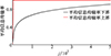 |
图1 平均信息传输率的上/下界与j的关系图 |
假设期望的平均信息传输率ξ为0.6, 则只需要得到 对应的j1以及
 对应的j2, j∈[j1, j2]。文献[16, 21-22]中调整矩阵同样设计为J=j·diag(2, 2, 1), 且j的选取按照上述方法完成。记本文设计的MMSE估计器为PSET, 文献[16]为ISET, 文献[21]为FSET, 文献[22]为SSET, 则不同平均信息传输率下, 4种MMSE估计器的j值如表 1所示。
不同平均信息传输率下4种估计器j的取值
根据表 1的结果, 下面进行第2个仿真实验, 设DDS-DNNS定位节点的期望轨迹为: 从(4, 0, 3.6)出发, 沿直线到(4, 5, 1.8), 再沿直线到(4, 0, 0)。定位节点期望轨迹如图 2所示。
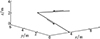 |
图2 定位节点期望轨迹图 |
设定位节点解算的局部坐标为(x(k), y(k), z(k)), 期望值为(xc(k), yc(k), zc(k)), 定义x, y, z坐标RMSE为
定位节点x坐标在ξ=0.2和ξ=0.8情景下的变化如图 3所示, 对应的RMSE变化如图 4所示; 定位节点y坐标在ξ=0.2和ξ=0.8情景下的变化如图 5所示, 对应的RMSE变化如图 6所示; 定位节点z坐标在ξ=0.2和ξ=0.8情景下的变化如图 7所示, 对应的RMSE变化如图 8所示。
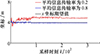 |
图3 定位节点坐标x在不同信息传输率下的变化 |
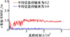 |
图4 定位节点坐标x的RMSE在不同信息传输率下的变化 |
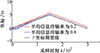 |
图5 定位节点坐标y在不同信息传输率下的变化 |
 |
图6 定位节点坐标y的RMSE在不同信息传输率下的变化 |
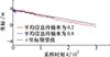 |
图7 定位节点坐标z在不同信息传输率下的变化 |
 |
图8 定位节点坐标z的RMSE在不同信息传输率下的变化 |
根据图 3~8可知: ①平均信息传输率越高, 定位节点的定位精度越高, 当ξ→1时, 估计器接收的测量值越来越多, MMSE估计器越来越接近标准KF形式; ②可调参数j能够有效调整平均信息传输率ξ, 因此本文设计的MMSE估计器能够针对不同应用场景需求, 调整对应需求的平均信息传输率。
下面进行第3个仿真实验, 对4种估计器性能的比较将从4个方面展开: ①定位精度rm的比较; ②估计误差协方差矩阵的迹tr(P(k|k))的比较; ③tr(P(k|k))稳态的采样时刻ks比较; ④1个采样周期内完成1次完整解算所消耗的时间tc比较。
定义定位精度rm为

对每一种MMSE估计器, 按照第2个仿真实验的环境, 依次令ξ=0.1, 0.2, …, 0.9, 得到4种估计器在不同平均信息传输率下的定位精度如图 9所示。
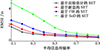 |
图9 不同平均信息传输率下4种估计器的定位精度比较 |
根据图 9可知: ①4种估计器在平均信息传输率ξ→1时, 定位精度几乎相同, 实际上4种估计器均为类KF形式的MMSE估计器, 只是触发机制不同; ②本文设计的MMSE估计器具有更好的定位精度, 尤其是在ξ较小时, 这说明了基于后验估计的SET机制能够有效选取对估计器重要的测量值。
令ξ=0.5, 按第2个仿真实验的环境, 4种估计器的tr(P(k|k))随采样时刻的变化如图 10所示。
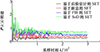 |
图10 ξ=0.5时4种估计器的tr(P(k|k))比较 |
根据图 10可知: ①4种估计器均满足稳定性, 且基于后验估计的MMSE估计器tr(P(k|k))稳态性能优于其他估计器; ②基于后验估计的MMSE估计器动态性能优于其他估计器, 且4种估计器tr(P(k|k))进入稳态的采样时刻不同。
受到ξ=0.5情景的启发, 定义tr(P(k|k))的平均值为 , 定义tr(P(k|k))进入稳态的采样时刻为ks, 定义采样周期[k, k+1)内完成1次完整解算所消耗的时间为tc(k), 1个采样周期内完成1次完整解算所消耗的时间tc=
 , 则4种估计器的P与ξ的关系如图 11所示; 4种估计器的ks与ξ的关系如图 12所示; 4种估计器的tc与ξ的关系如图 13所示。
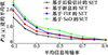 |
图11 不同平均信息传输率下4种估计器的P比较 |
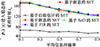 |
图12 不同平均信息传输率下4种估计器的ks比较 |
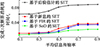 |
图13 不同平均信息传输率下4种估计器的tc比较 |
根据图 11~13可知: ①当平均信息传输率ξ→1时, 4种估计器的P趋于一致; ②当ξ较小时, 本文设计的MMSE估计器的P明显小于其他3种估计器; ③本文设计的MMSE估计器ks受ξ的影响不大, 而其他3种估计器ks的变化几乎相同, 实际上, 其他3种估计器的SET机制只需要考虑当前时刻的测量值, 因此随着ξ的增大, 接收到的测量值信息越多, 从而更早进入稳态。另一方面, 通过(38)式可知, 基于后验估计的SET不仅要考虑当前时刻测量值, 而且要考虑二阶矩信息。因此即使在ξ较小时, 估计器仍然能够通过二阶矩信息有效筛选出对一步预测修正重要的信息, 从而使得本文设计的MMSE估计器能够更早进入稳态; ④尽管二阶矩信息使得本文设计的MMSE估计器的tr(P(k|k)), P与ks均具备更好的解算效果, 但是tc明显大于其他3种估计器。
最后进行第4个仿真实验, 通过Monte Carlo模拟来获取平均信息传输率与g(k)的关系。设模拟次数为500, 定义 , 依次令ξ=0, 0.1, 0.2, …, 0.9, 则g与ξ的关系如图 14所示。
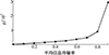 |
图14 g与平均信息传输率的关系图 |
根据图 14可知: ①当ξ→1时, g越来越大, 这说明了平均信息传输率较大时, 一阶矩信息‖δ(k)‖KT(k)JK(k)2占主导地位, 二阶矩信息ρ(k)对SET机制的影响程度非常小; ②当ξ较小时, ‖δ(k)‖KT(k)JK(k)2和ρ(k)对SET机制均有影响, ξ→0时, g趋近于1。因此,一阶矩信息‖δ(k)‖KT(k)JK(k)2对SET机制的影响是主要的, 二阶矩信息ρ(k)只有在ξ较小时才与一阶矩信息共同影响SET机制。
4 结论
1) Bayes理论下具有SET机制的MMSE估计器在不同的平均信息传输率下均能较好地完成状态估计, 例如ξ=0.2时, PSET定位精度为1.132 m, 而ISET定位精度为1.508 m, FSET为2.117 m, SSET为4.005 m; ξ=0.8时, PSET定位精度为0.501 m, 而ISET定位精度为0.546 m, FSET为0.649 m, SSET为0.840 m。
2) 后验估计是估计中最全面的信息, 基于后验估计的SET机制能够选出对估计器重要的测量值。
3) PSET与ISET、FSET、SSET最大的区别在于二阶矩信息, 且当平均信息传输率较小时, 一阶矩信息和二阶矩信息均对SET机制有影响, 而当平均信息传输率增大时, 二阶矩信息对SET机制的影响程度越来越小。
4) 由于对二阶矩信息的利用, 通过PSET推导得到的MMSE估计器从定位精度、动态性能、稳态性能的角度出发具备更好的估计效果。与此同时, 二阶矩信息的利用增大了估计器的计算复杂度, 如何降低估计器的计算复杂度并将结论推广至多节点情景是下一步研究的重点。
5) 通过对平均信息传输率上界和下界的推导, 为调整矩阵的选取提供理论依据, 且仿真实验证明, 调整矩阵能够有效调整平均信息传输率。
6) 本文估计器针对的是系统噪声和量测噪声满足Gaussian性的系统模型。对于非Gaussian噪声、能量有界噪声、幅值有界噪声等复杂噪声环境下的SET机制设计是下一步研究中需要考虑的问题。
References
- Gao Chao, Lu Jianhua, Zhao Guorong, et al. Decentralized navigational state estimation for networked navigation systems with finite channel capacity and randomly switching topologies[J]. Aerospace Engineering, 2018, 232(2): 201–214 [Google Scholar]
- Hu Zhongyao, Chen Bo, Wan Rusheng, et al. Multi-sensor state estimation with a sequential stochastic event-triggered mechanism[J]. IEEE Trans on Signal and Information Processing over Networks, 2025, 11(1): 342–352 [Google Scholar]
- Liu Wei. Event-triggered state estimation through confidence level[J]. IEEE Trans on Signal Processing, 2025, 73(2): 1337–1350 [Google Scholar]
- Meng Rui, Hua Changchun, Li Kuo, et al. Estimated states-based event-triggered control for interconnected nonlinear systems with hybrid stochastic faults[J]. IEEE Trans on Systems, Man, and Cybernetics: Systems, 2025, 55(4): 3064–3073. [Article] [Google Scholar]
- Grigorescu A, Boche H, Schaefer R F, et al. Capacity of finite state channels with feedback: algorithmic and optimization theoretic properties[J]. IEEE Trans on Information Theory, 2024, 70(8): 5413–5426. [Article] [Google Scholar]
- Li Feng, Wang Yanan, Shen Hao. Dual event-triggered synchronization of two-time-scale jumping neural networks and its application in image encryption and decryption[J]. IEEE Trans on Network Science and Engineering, 2025, 12(2): 943–954. [Article] [Google Scholar]
- Liu Jia, Liu Jiapeng, Wang Qingguo, et al. Adaptive neural network finite-time event triggered intelligent control for stochastic nonlinear systems with time-varying constraints[J]. IEEE Trans on Artificial Intelligence, 2025, 6(3): 773–779. [Article] [Google Scholar]
- Zhao Guorong, Han Xu, Wang Kang. Offline state estimator with sensor gain degradation, transmission delay, and packet loss[J]. Acta Automatica Sinica, 2020, 46(3): 540–548 (in Chinese) [Google Scholar]
- Zhang Xianming, Han Qinglong, Zhang Baolin. An overview and deep investigation on sampled-data-based event-triggered control and filtering for networked systems[J]. IEEE Trans on Industrial Informatics, 2017, 13(1): 4–16. [Article] [Google Scholar]
- Wu Junfeng, Jia Qingshan, Johansson K H, et al. Event-based sensor data scheduling: trade-off between communication rate and estimation quality[J]. IEEE Trans on Automatic Control, 2013, 58(4): 1041–1046. [Article] [Google Scholar]
- You Keyou, Xie Lihua. Kalman filtering with scheduled measurements[J]. IEEE Trans on Signal Processing, 2013, 61(6): 1520–1530. [Article] [Google Scholar]
- Shi Dawei, Chen Tongwen, Shi Lin. On set-valued Kalman filtering and its application to event-based state estimation[J]. IEEE Trans on Automatic Control, 2015, 60(5): 1275–1290. [Article] [Google Scholar]
- Shi D, Chen T, Shi L. An event-triggered approach to state estimation with multiple point-and set-valued measurements[J]. Automatica, 2014, 50(6): 1641–1648. [Article] [Google Scholar]
- Trimpe S, Andrea R D. Event-based state estimation with variance-based triggering[J]. IEEE Trans on Automatic Control, 2014, 59(12): 3266–3281. [Article] [Google Scholar]
- He Lidong, Chen Jiming, Qi Yifei. Event-based state estimation: optimal algorithm with generalized closed skew normal distribution[J]. IEEE Trans on Automatic Control, 2019, 64(1): 321–328. [Article] [Google Scholar]
- Han Duo, Mo Yilin, Wu Junfeng, et al. Stochastic event-triggered sensor schedule for remote state estimation[J]. IEEE Trans on Automatic Control, 2015, 60(10): 2661–2675. [Article] [Google Scholar]
- Xu Liang, Mo Yilin, Xie Lihua. Remote state estimation with stochastic event-triggered sensor schedule and packet drops[J]. IEEE Trans on Automatic Control, 2020, 65(11): 4981–4988. [Article] [Google Scholar]
- Mohammadi A, Plataniotis K N. Event-based estimation with information-based triggering and adaptive update[J]. IEEE Trans on Signal Processing, 2017, 65(18): 4924–4939. [Article] [Google Scholar]
- Huang Jiarao, Shi Dawei, Chen Tongwei. Event-triggered state estimation with an energy harvesting sensor[J]. IEEE Trans on Automatic Control, 2017, 62(9): 4768–4775. [Article] [Google Scholar]
- Deng Di, Xiong Junlin. Kalman-like filter for event-triggered remote state estimation over an additive noise channel[J]. IEEE Control Systems Letters, 2024, 8(11): 205–210 [Google Scholar]
- Alavi S A, Mehran K, Hao Yang. Optimal observer synthesis for microgrids with adaptive send-on-delta sampling over iot communication networks[J]. IEEE Trans on Industrial Electronics, 2021, 68(11): 11318–11327. [Article] [Google Scholar]
- Schmitt E J, Noack B, Krippner W, et al. Gaussianity-preserving event-based state estimation with an FIR-based stochastic trigger[J]. IEEE Control Systems Letters, 2019, 3(3): 769–774. [Article] [Google Scholar]
- Hu Zhongya, Chen Bo, Wang Rusheng. Remote state estimation with posterior-based stochastic event-triggered schedule[J]. IEEE Trans on Automatic Control, 2024, 69(2): 1194–1201. [Article] [Google Scholar]
- Chundawat V S, Tarun A K, Mandal M, et al. A universal metric for robust evaluation of synthetic tabular data[J]. IEEE Trans on Artificial Intelligence, 2024, 5(1): 300–309. [Article] [Google Scholar]
- Shi Bao, Liu Xiaolei, Gai Mingjiu, et al. Fundamental to practical matrix analysis[M]. Beijing: National Defence Industry Press, 2017. (in Chinese) [Google Scholar]
- Chen Chuncheng, Song Zhiyuan, Wu Keer, et al. A novel solution for solving time-varying algebraic riccati equations and its application to sound source tracking[J]. IEEE Sensors Journal, 2025, 25(7): 11155–11166. [Article] [Google Scholar]
- Zhang Liyang, Chen Xinlei, Lu Lichang, et al. Efficient solution of wideband partial modification problem via wideband Sherman-Morrison-Woodbury algorithm[J]. IEEE Antennas and Wireless Propagation Letters, 2024, 23(12): 4862–4866. [Article] [Google Scholar]
- Qu Z. Robust control of a class of nonlinear uncertain systems[J]. IEEE Trans on Automatic Control, 1992, 37(9): 1437–1442. [Article] [Google Scholar]
- Zou Lang, Liu Xiangbin, Su Hongye, et al. Learning-based robust adaptive rapid exponential stabilization for a class of nonlinear CPSs under DoS attacks[J]. IEEE Trans on Systems, Man, and Cybernetics: Systems, 2025, 55(3): 1898–1911. [Article] [Google Scholar]
- Olkin I, Pukelsheim F. The distance between two random vectors with given dispersion matrices[J]. Linear Algebra and Its Applications, 1982, 48(1): 257–263 [Google Scholar]
All Tables
All Figures
|
图1 平均信息传输率的上/下界与j的关系图 |
| In the text | |
|
图2 定位节点期望轨迹图 |
| In the text | |
|
图3 定位节点坐标x在不同信息传输率下的变化 |
| In the text | |
|
图4 定位节点坐标x的RMSE在不同信息传输率下的变化 |
| In the text | |
|
图5 定位节点坐标y在不同信息传输率下的变化 |
| In the text | |
|
图6 定位节点坐标y的RMSE在不同信息传输率下的变化 |
| In the text | |
|
图7 定位节点坐标z在不同信息传输率下的变化 |
| In the text | |
|
图8 定位节点坐标z的RMSE在不同信息传输率下的变化 |
| In the text | |
|
图9 不同平均信息传输率下4种估计器的定位精度比较 |
| In the text | |
|
图10 ξ=0.5时4种估计器的tr(P(k|k))比较 |
| In the text | |
|
图11 不同平均信息传输率下4种估计器的P比较 |
| In the text | |
|
图12 不同平均信息传输率下4种估计器的ks比较 |
| In the text | |
|
图13 不同平均信息传输率下4种估计器的tc比较 |
| In the text | |
|
图14 g与平均信息传输率的关系图 |
| In the text | |
Current usage metrics show cumulative count of Article Views (full-text article views including HTML views, PDF and ePub downloads, according to the available data) and Abstracts Views on Vision4Press platform.
Data correspond to usage on the plateform after 2015. The current usage metrics is available 48-96 hours after online publication and is updated daily on week days.
Initial download of the metrics may take a while.